

Ambient noise tomography beneath Greenland ice
Imaging concealed geology with passive seismic methods: a case study from Greenland.
The challenge of finding the next generation of mineral deposits
Mineral exploration is facing a fundamental challenge. The world needs increasing quantities of copper and other metals, yet finding new deposits is becoming progressively more difficult.
Copper illustrates the scale of the problem. Global annual demand could approximately double over the next 25 years, reaching 50 million tonnes by 2050, if net-zero emission targets are to be met (Cathles et al. 2025, cited in Schodde 2025). At the same time, the number of significant mineral discoveries has declined, and the cost of making those discoveries has increased substantially.
According to an analysis by Richard Schodde (2025), significant mineral discoveries worldwide peaked at 202 in 2009 and have since declined to approximately 70–90 per year. The estimated cost of discovering a significant deposit has risen from about US$65 million during 1980–1999 to approximately US$200 million today, expressed in constant dollars.
Part of the explanation is geological. For much of the twentieth century, exploration concentrated on mineral deposits that were exposed at the surface or could be identified from visible geological features. Many of these relatively accessible deposits have now been discovered.
The next generation of discoveries will increasingly come from deeper geological environments or from deposits concealed beneath sedimentary formations, volcanic rocks, glacial deposits and other types of cover.
The historical record already shows this shift. From the 1950s to the 1980s, copper deposits were found on average 50–70 metres below the surface; in the 1990s and 2000s, about 110 metres; between 2010 and 2019, 202 metres. The average depth of a copper discovery doubled in a single decade. Zinc–lead discoveries followed the same course, from 29 metres in the 1950s to 234 metres in the 2010s (Schodde 2025).
Depth also changes which methods work. Below about 50 metres, geophysics becomes the main tool for deciding where to drill; below about 500 metres of cover, its effectiveness currently drops off, and targeting relies mainly on extrapolation from known ore and on deep drilling (Schodde 2025). Finding the next deposits will therefore depend on imaging the geology beneath the cover, at the depths where discoveries are now made.
Greenland: testing seismic imaging beneath the ice
Greenland provides an unusual example of the challenges associated with exploration beneath cover.
Approximately 80% of its surface is covered by ice, which in some regions reaches several kilometres in thickness (Figure 1). The island contains a wide range of mineral resources, including many materials considered critical for modern technologies.
Nearly all known mineral deposits lie along the ice-free margins, because that is where the geology can be mapped and explored. Beneath the ice, the geology is poorly known, largely extrapolated from rocks exposed near the coast, and exploration is difficult.
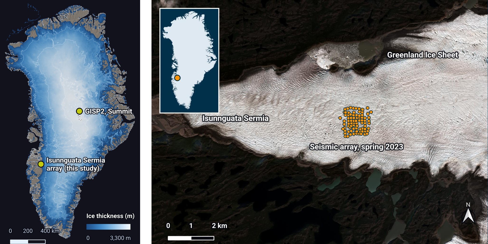
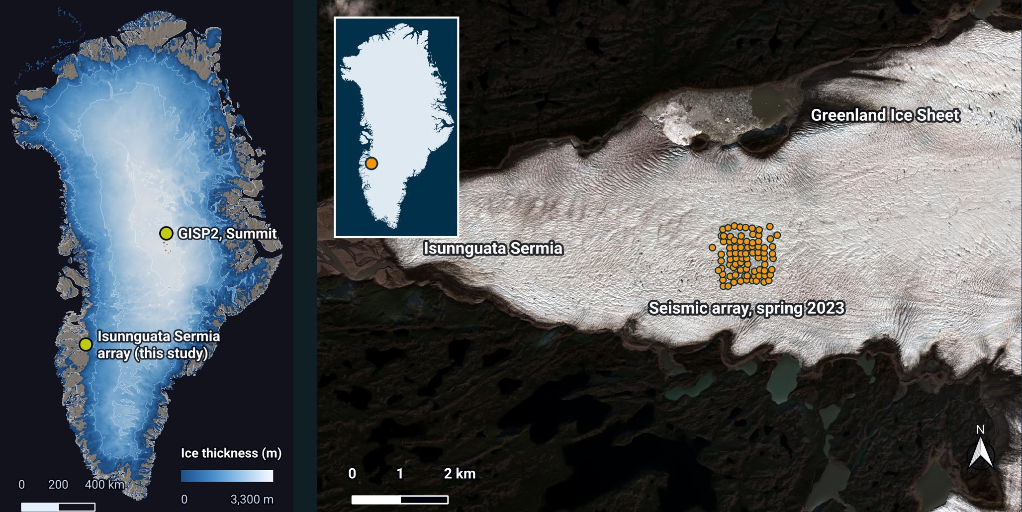
Can the ground beneath a glacier be explored efficiently by methods other than drilling, or by methods that guide drilling and make it more efficient? We tested ambient noise tomography, a passive seismic method, on recordings from an existing seismic array on Isunnguata Sermia, a glacier in western Greenland.
The method needs no explosives or vibrators. It measures how fast the seismic waves that continuously travel through the ground pass from one sensor to the next; longer waves sample greater depths. It therefore depends on two conditions: the sensors must record these waves well, and the waves must reach the rock beneath the cover and carry its signature back to the surface. On a glacier, neither condition can be taken for granted, and the study asked two questions.
First, is the signal recorded on a glacier good? The sensors are coupled to moving, fracturing ice, and icequakes add energy of their own.
Second, could the ice impede the transmission of seismic energy and mask the ground below it? The strong contrast between ice and rock, and the crevasses that cut the ice, might limit what can be imaged beneath the bed.
Key results
From 35 days of recordings at 82 stations, over ice 330–650 metres thick, the answers are: the signal is good, and the ice does not mask the ground below it.
- Q1 · Signal qualityThe noise on the glacier is strong across the band of interest, relatively homogeneous and arrives from many directions: the conditions ambient noise tomography needs.
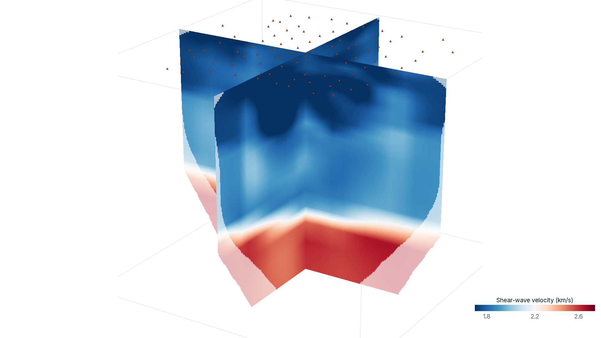
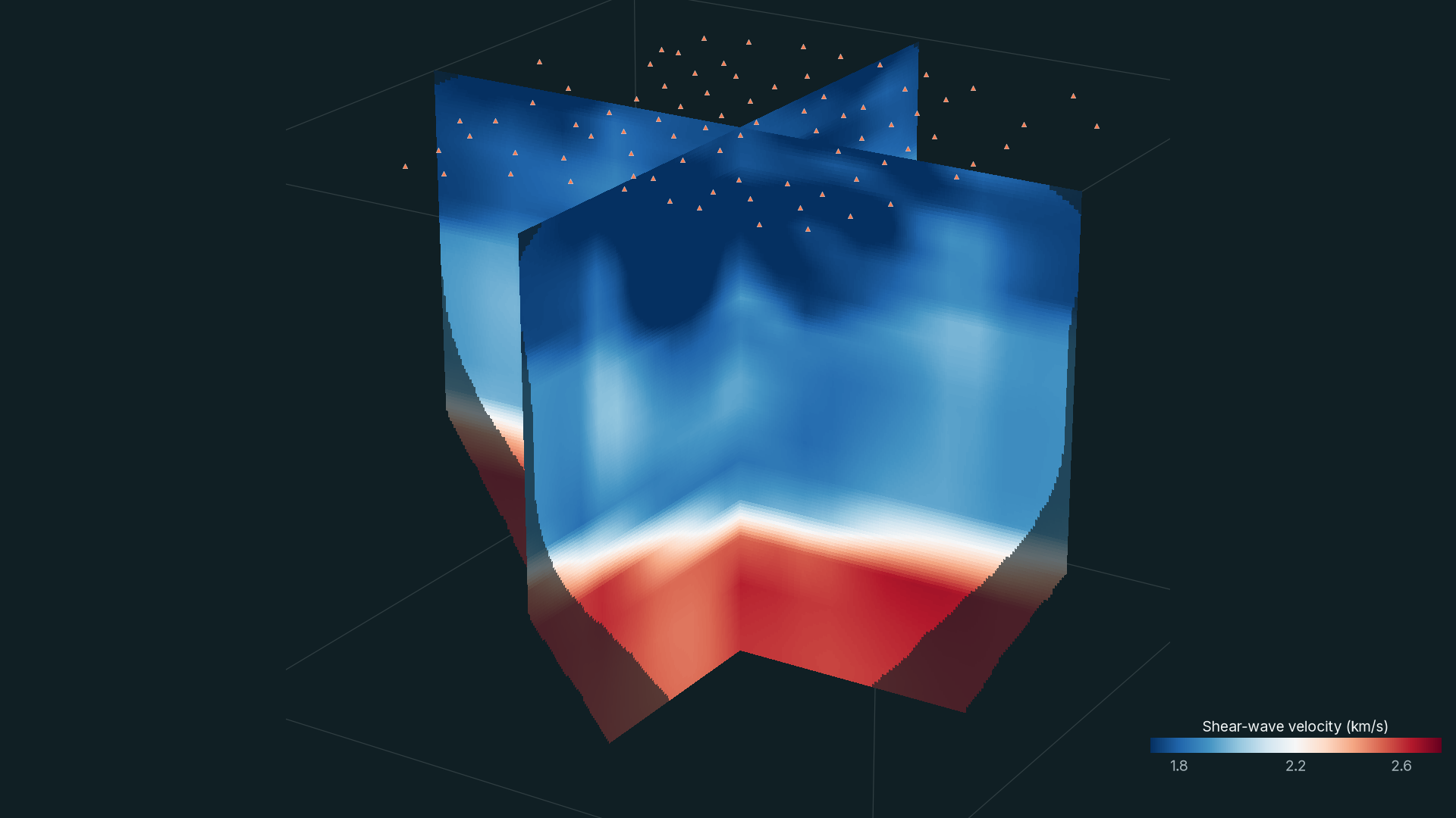
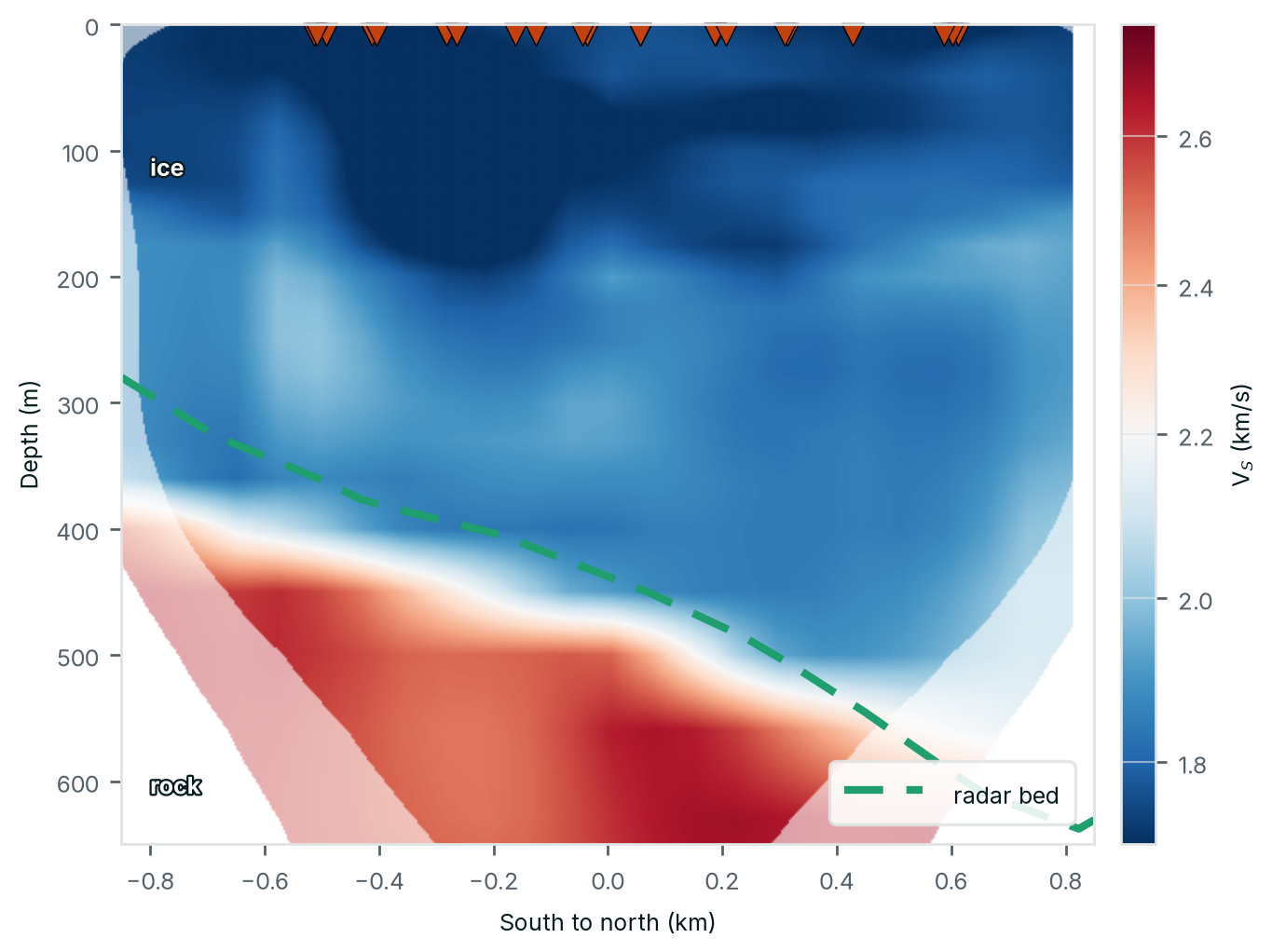
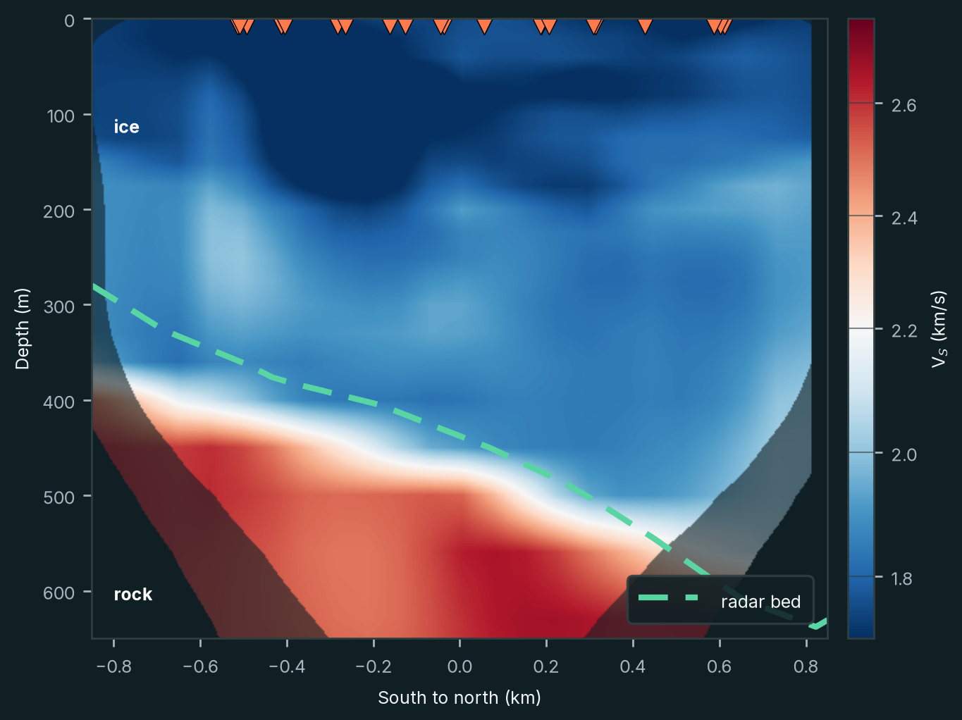
- Q2 · Seeing beneath the iceThe ice does not prevent the seismic waves from sampling the rock beneath it: the velocity model shows slow ice over faster rock (Figure 2).
- The ice–rock transitionThe transition in the velocity model agrees with independent radar measurements: 436 metres deep on average, against 435 metres from radar.
- CoverageDespite the array's small aperture, the model resolves the transition over 87% of the array's footprint.
- VelocitiesThe ice, at 1.73–1.90 km/s, lies within the range measured on glaciers (1.70–1.95 km/s; Podolskiy and Walter 2016); the rock beneath is faster, about 2.6 km/s.
- Structure within the iceThe model captures velocity variations within the ice: a slower upper layer over a faster lower one, and a dependence on direction aligned with the crevasses.
The rest of this article explains how these results were obtained.
Seeing beneath the surface
Traditional mineral exploration relies heavily on geological mapping, surface geochemistry and direct sampling. These methods remain essential, but their effectiveness decreases when the geology of interest is concealed.
Drilling provides direct observations of the subsurface, but it is expensive and samples only a small volume of rock. Without sufficient geological information, drilling can become an inefficient way of testing exploration hypotheses.
Geophysical methods help address this problem by measuring physical properties that vary between geological formations. Gravity, magnetic, electromagnetic and seismic measurements each provide different information about the subsurface.
Seismic imaging is particularly interesting because seismic-wave velocities depend on the mechanical properties of rocks. Variations in velocity can reveal geological boundaries, faults and changes in rock properties, helping geologists understand the three-dimensional architecture of a mineral system.
The difficulty is that conventional seismic surveys often require an artificial energy source, such as explosives or mechanical vibrators. These surveys can be costly and logistically challenging, particularly in remote areas with difficult terrain.
Passive seismic methods offer another approach. Rather than generating seismic waves, they use energy already present in the environment.
Listening to the Earth's natural vibrations
The ground is never completely still. Ocean waves, wind, rivers, industrial activity and many other processes continuously generate weak seismic vibrations. On a glacier, icequakes add many more: the Greenland array detected nearly 19,000 small seismic events in 35 days, almost all within the ice.
These signals are generally too small to be felt, but modern seismic instruments can measure them with considerable precision.
Ambient noise tomography (ANT) takes advantage of this naturally occurring seismic energy. By comparing recordings from pairs of seismic stations, it is possible to extract information about the propagation of seismic waves between them.
The underlying principle is known as seismic interferometry. When sufficiently long recordings are correlated, the resulting signal can approximate part of the seismic response that would be observed if a source were placed at one station and recorded at the other.
The velocity of these waves varies with frequency. Longer-period waves generally sample deeper parts of the subsurface, while shorter-period waves are more sensitive to shallow structures.
By measuring this variation across many station pairs, we can reconstruct a three-dimensional model of seismic velocity (Figure 3).
The method has an important practical advantage: seismic instruments can record continuously without requiring an artificial seismic source. Arrays can be deployed in remote regions and left to acquire data autonomously for several weeks.
For mineral exploration beneath cover, this creates opportunities to investigate geological structures that are difficult to access using conventional methods.
An existing experiment in Greenland
In spring 2023, a research team led by Florent Gimbert and colleagues at Université Grenoble Alpes installed 82 seismic stations on Isunnguata Sermia, a glacier in western Greenland.
The instruments were distributed across an array approximately 1.6 kilometres wide, with an average spacing of 110 metres. They recorded continuously for 35 days.
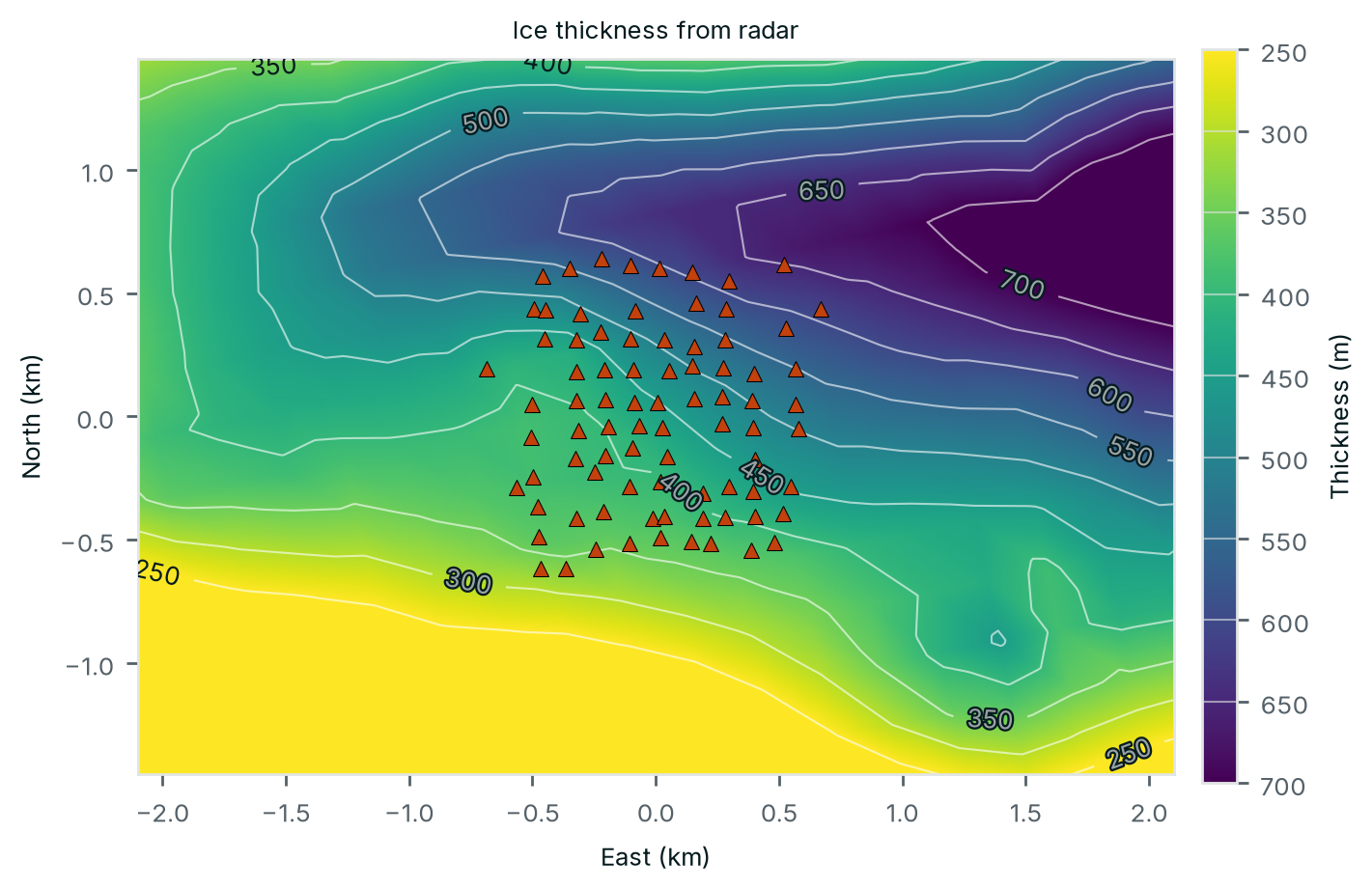
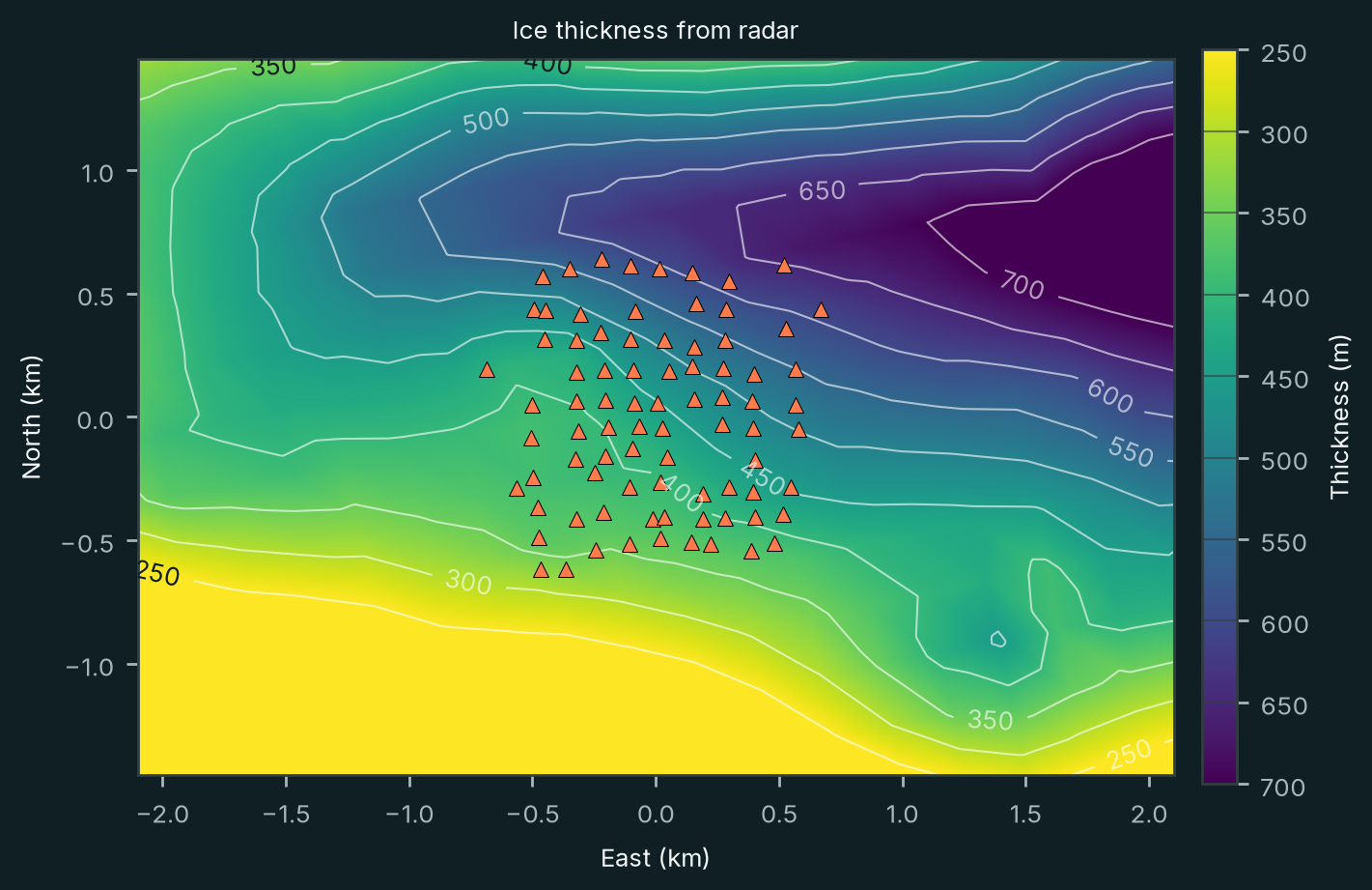
Beneath the array, radar measurements indicated that the ice was between 330 and 650 metres thick (Figure 4).
The original purpose of the experiment was to study glacier dynamics. However, the recordings also provided an opportunity to investigate whether passive seismic methods could image the rock beneath the ice.
Working with our colleagues at Université Grenoble Alpes, we used these recordings to answer the two questions.
The ambient seismic wavefield recorded by the array
The ambient noise field on Isunnguata Sermia is excellent, in part because of the glacier's own activity. As ice flows, it deforms and fractures. Crevasses open, blocks move and the glacier interacts mechanically with the rock beneath it. These processes generate numerous seismic signals, including small earthquakes within the ice.
The glacier is not the only source. Its signals add to those that reach the array from elsewhere; the ocean microseism, for example, appears at every station.
The noise has the properties ambient noise tomography needs (Figure 5). It is strong across the band of interest: energy was present in every hour of the 35 days from about 1.5 to 15 Hz, which spans the 2.2–12 Hz of the dispersion measurements. It is relatively homogeneous: over that band, half of all 60,592 station-hours lie within about 6 dB of each other. And it comes from multiple directions: at 2.5–5 Hz it arrives from most azimuths, strongest from the north and south-southeast, so no single source region dominates.
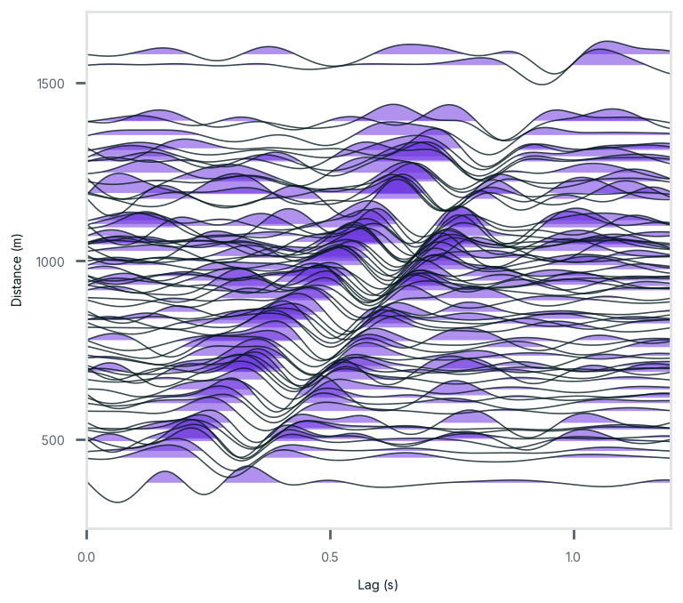
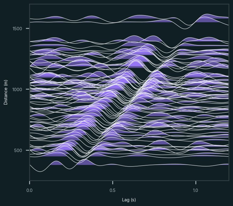
Correlating the recordings of the 3,321 station pairs therefore gives coherent signals. The correlations show a clean moveout: their arrivals move away from zero lag as the distance between stations grows, at about 1.6–1.8 km/s. Combined over all pairs, they give a well-defined dispersion curve, from 2.2 to 12 Hz at 1.6–2.0 km/s.
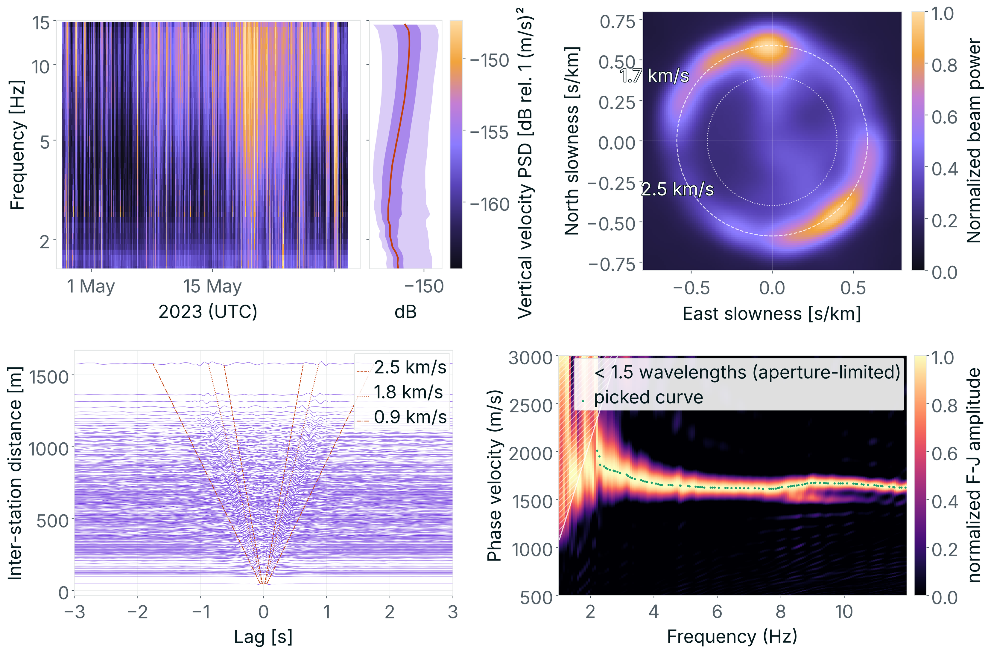
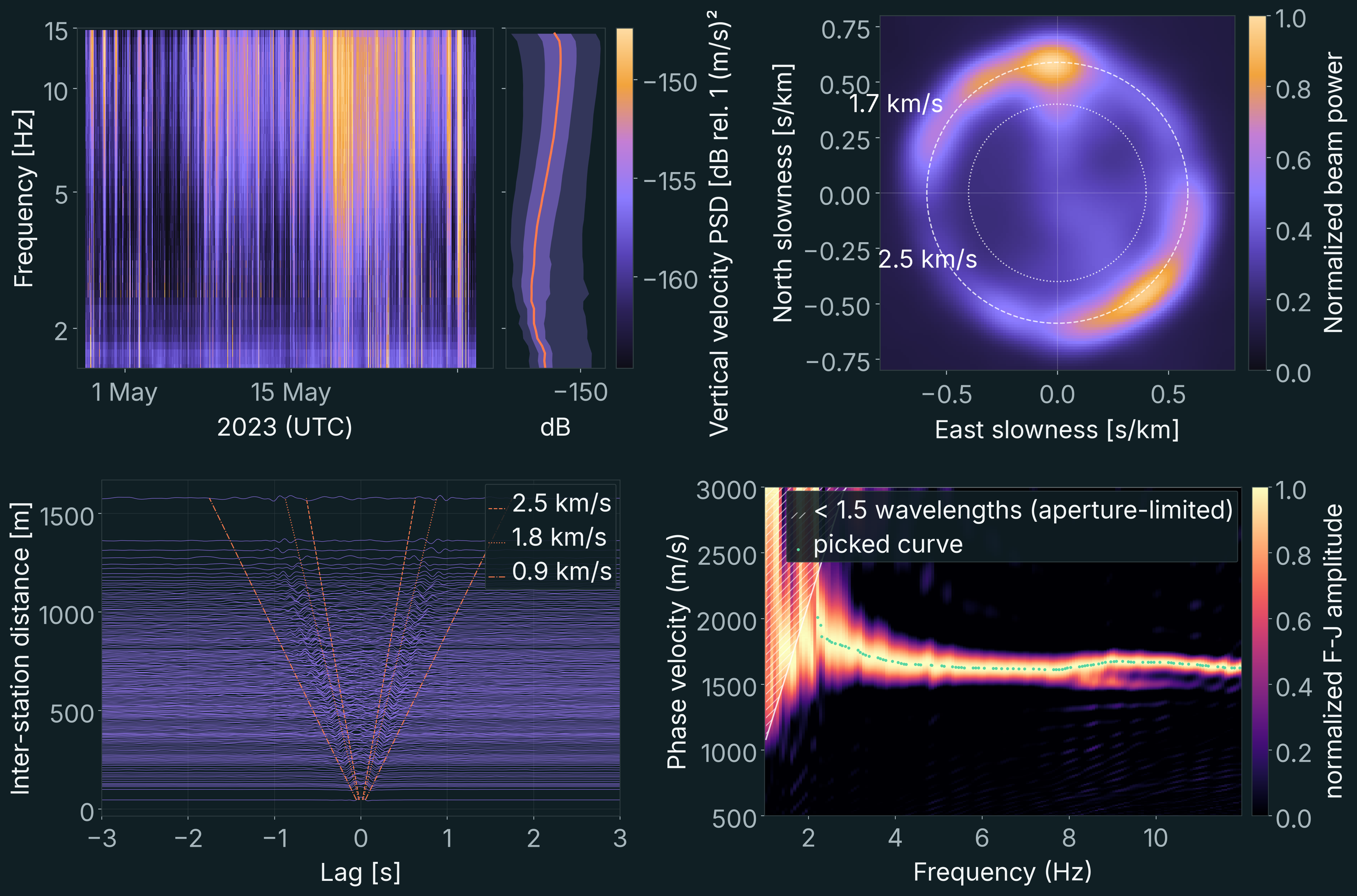
This answers the first question: the signal recorded on the glacier is good and, even with the array's small aperture, suitable for inversion.
Inversion strategy
The second question was whether we could image the bedrock below the glacier. We pushed the dataset to its limits: despite the array's small aperture, we tried to recover not only the velocity contrast between ice and rock, but also the topography of the bed and the structure within the ice.
To do so, we solved a simple problem first and increased the complexity little by little, toward a full three-dimensional model (Figure 6). Each step adds observations or model complexity, and starts from the model of the step before:
- Whole-array dispersion to a 1-D model. One Rayleigh-wave and one Love-wave curve, averaged over the whole array; five unknowns: three velocities and two layer thicknesses.
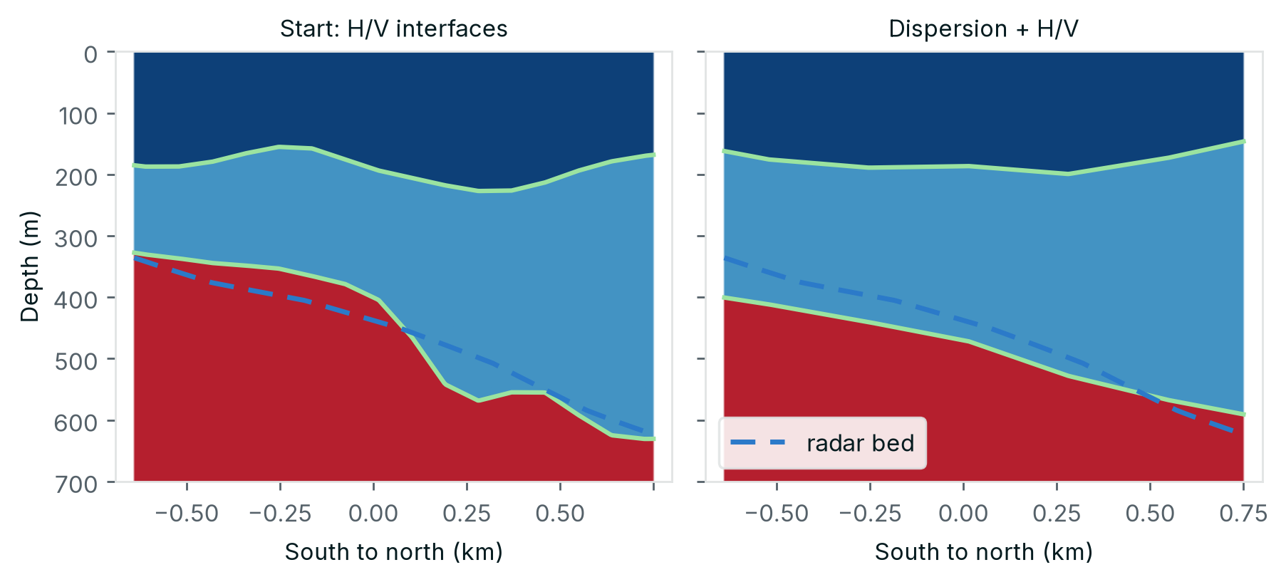
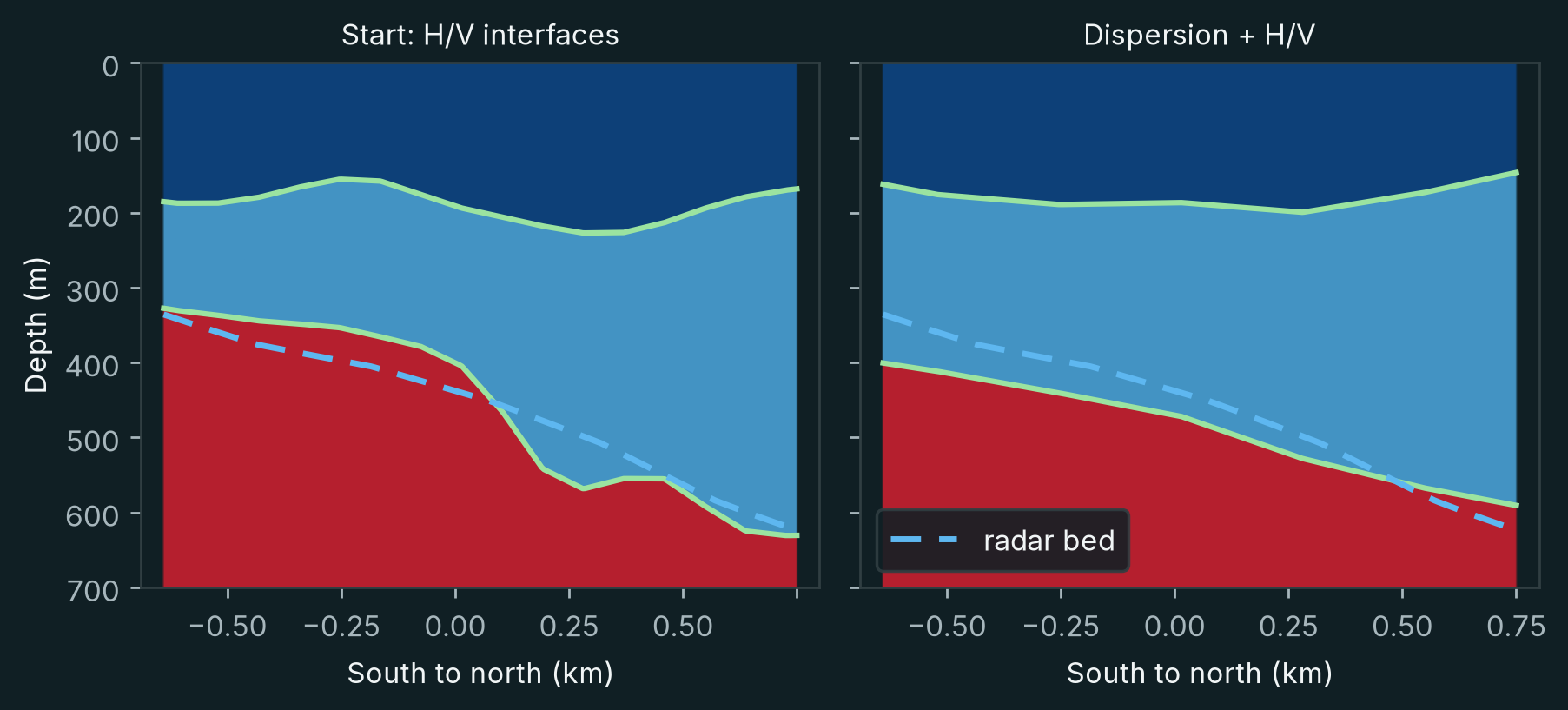
- H/V peaks to 3-D interfaces. The H/V peaks at each station, assigned to the interfaces by the 1-D model; the unknowns are the shapes of two interfaces.
- Dispersion and H/V peaks to refined interfaces. Dispersion between station pairs and the H/V peaks together; the unknowns are the two interfaces in 3-D.
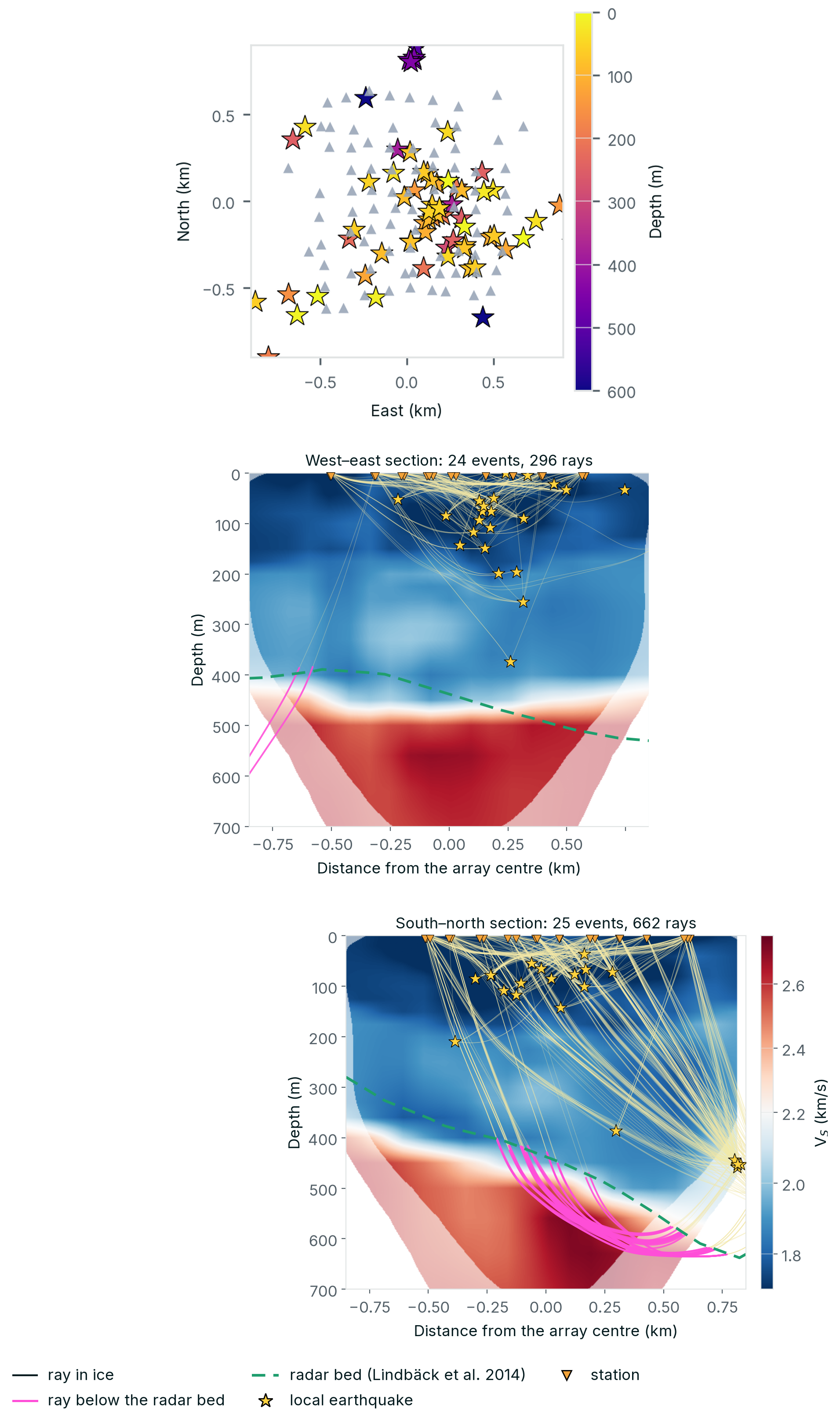
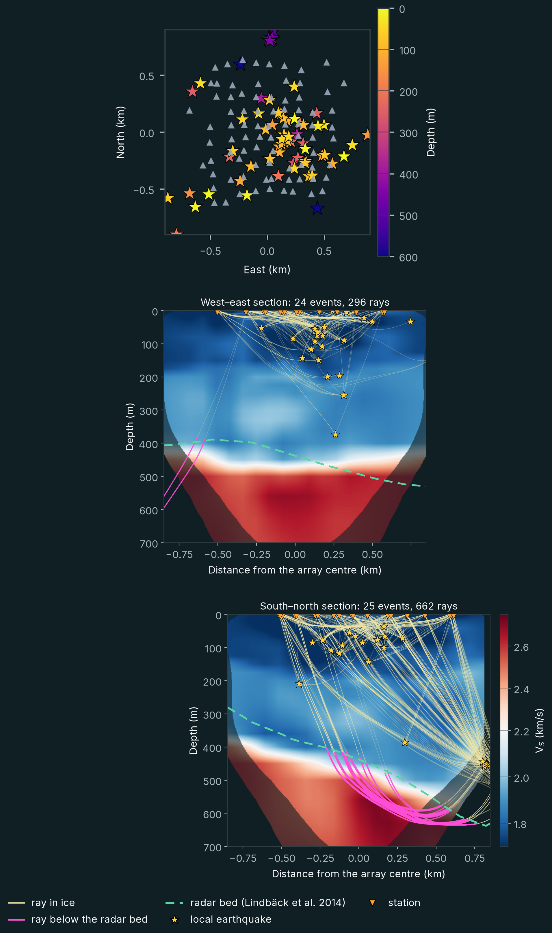
- Dispersion and local earthquakes to a 3-D velocity model. Dispersion and earthquake arrival times; the unknowns are shear and P-wave velocity in 3-D and the 71 hypocentres.
- Full-waveform inversion. The correlation waveforms themselves, 2–9 Hz; the unknown is shear velocity in 3-D, with every waveform simulated.
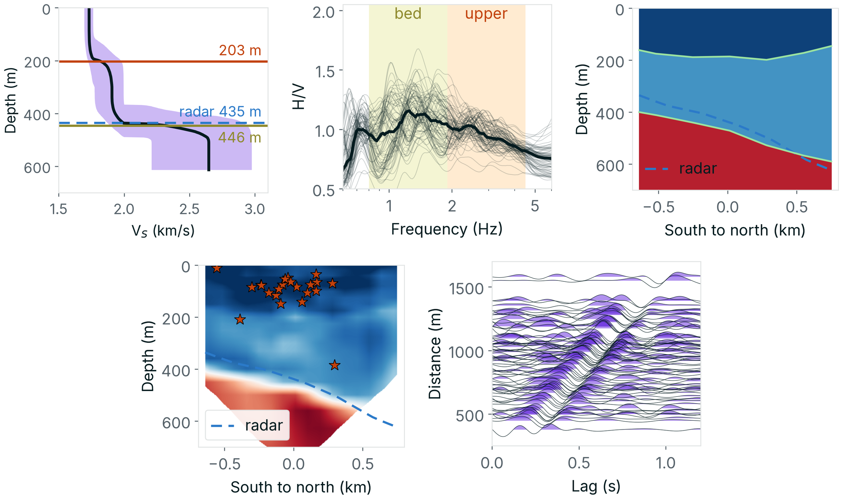
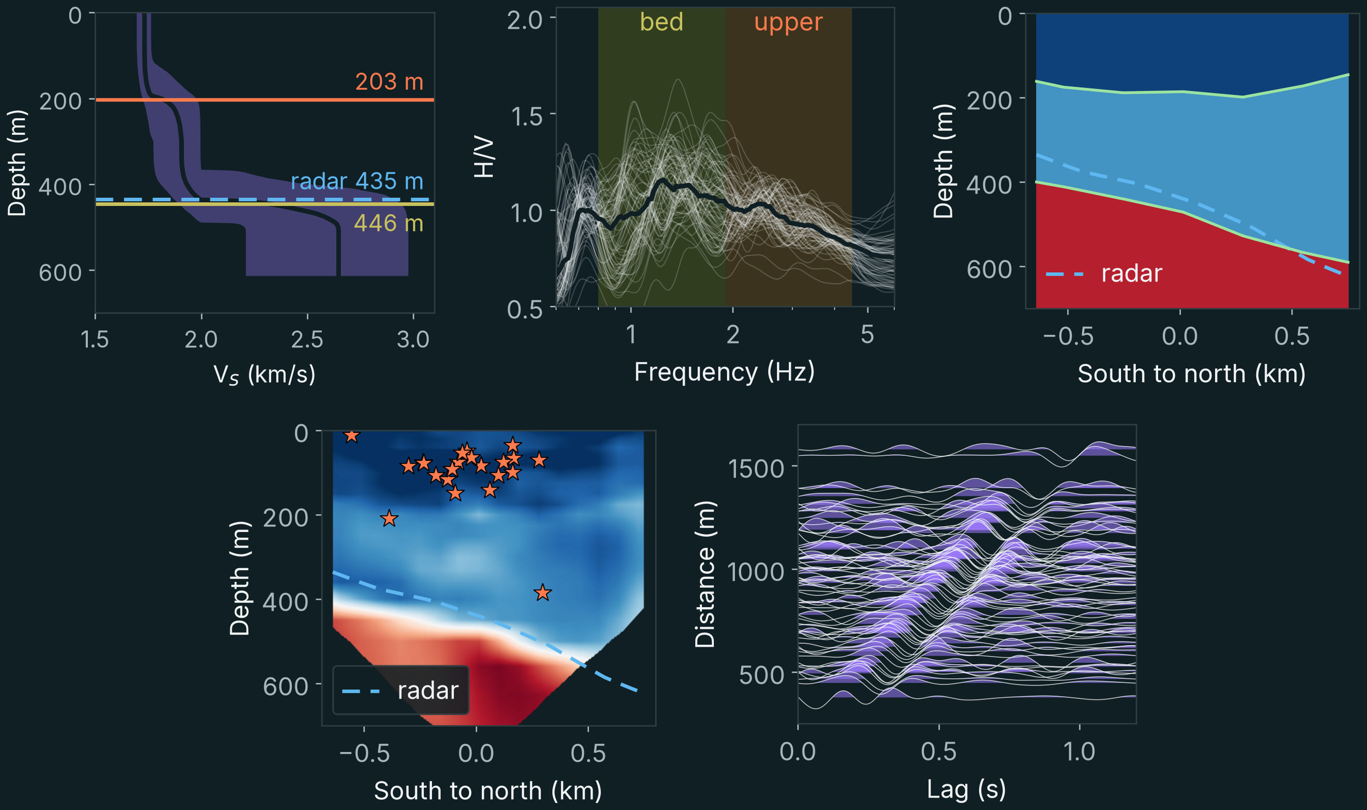
The sections below take each step in turn.
Step 1: whole-array dispersion to a 1-D model
We began with a relatively simple representation of the subsurface, assuming that seismic velocity varied only with depth.
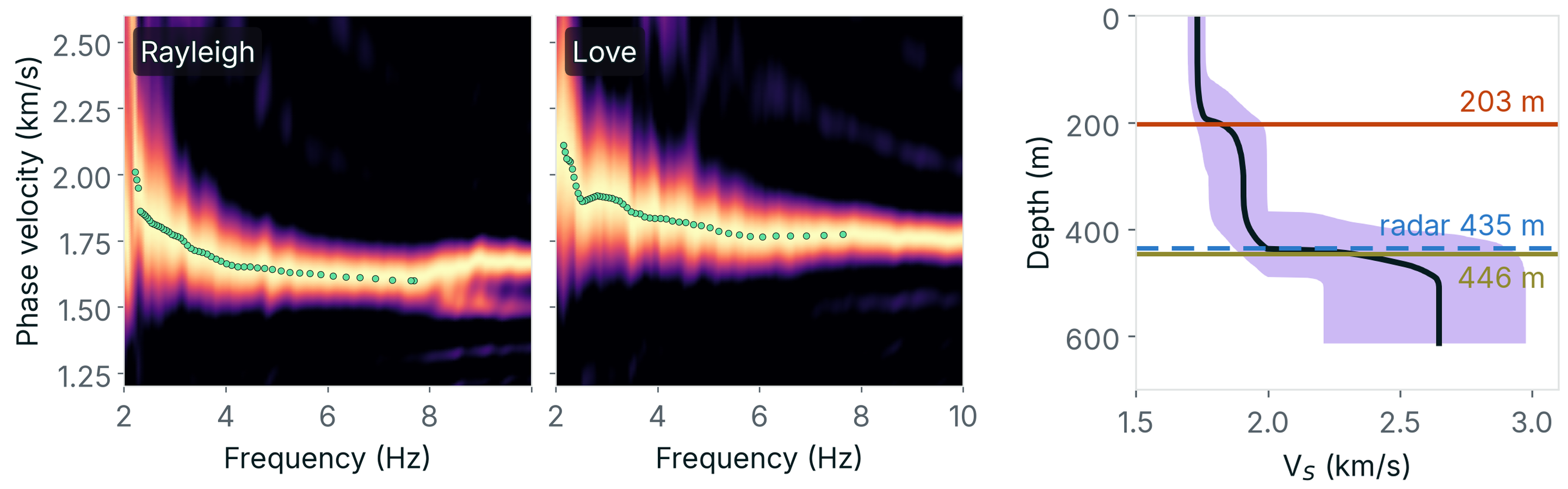
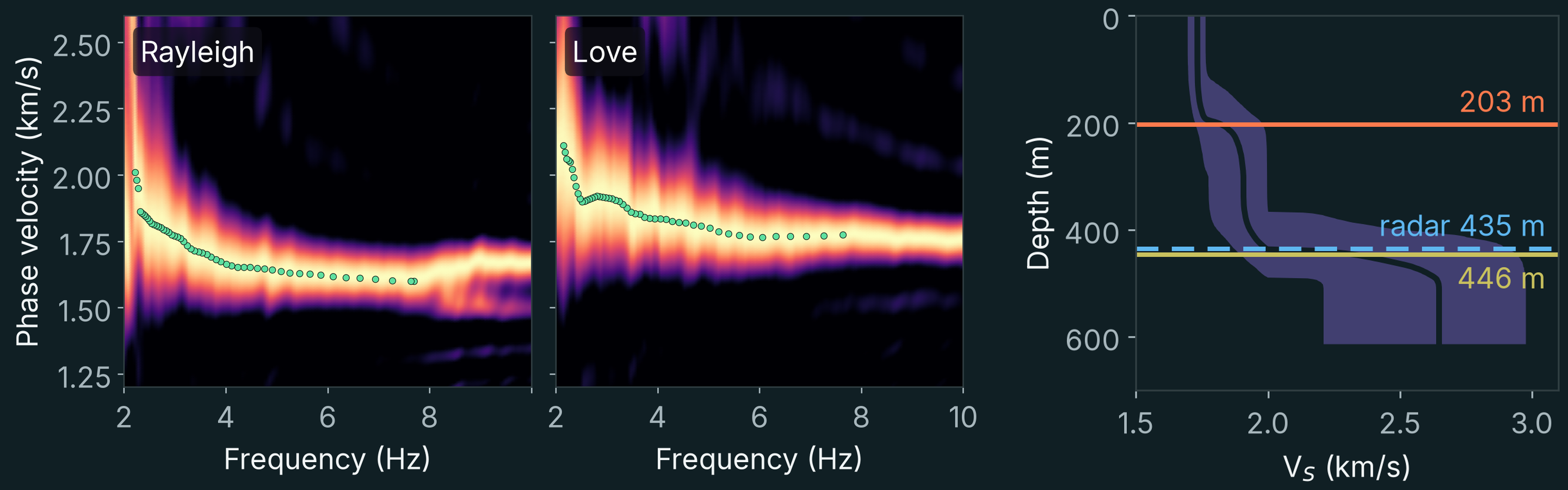
The measurements indicated two layers within the ice, with shear-wave velocities of approximately 1.73 and 1.90 kilometres per second. Beneath them, velocity increased to about 2.63 kilometres per second, consistent with the transition from ice to solid bedrock.
The resulting model placed the ice–bedrock boundary at a depth of 436 metres (95% range 367–489 metres; Figure 7).
Independent radar measurements indicated a median ice thickness of 435 metres beneath the stations.
The agreement was remarkable, particularly because the radar information had not been used to constrain the seismic inversion.
Step 2: H/V peaks to 3-D interfaces
Of course, the glacier does not rest on a flat bedrock surface. Its thickness varies substantially across the array.
To investigate these variations, we examined the relative amplitudes of horizontal and vertical seismic motion, a measurement known as the horizontal-to-vertical spectral ratio, or HVSR.
This ratio is sensitive to contrasts in seismic properties between layers. Its peaks fall at frequencies set by the depths of the interfaces beneath each station: the deeper the interface, the lower the frequency. The 1-D model tells which peaks belong to which interface; the peaks then give the shape of each interface across the array (Figure 8).
The seismic measurements indicated that the bedrock deepened towards the north by approximately 180 metres per kilometre. Radar observations gave a corresponding gradient of 188 metres per kilometre.
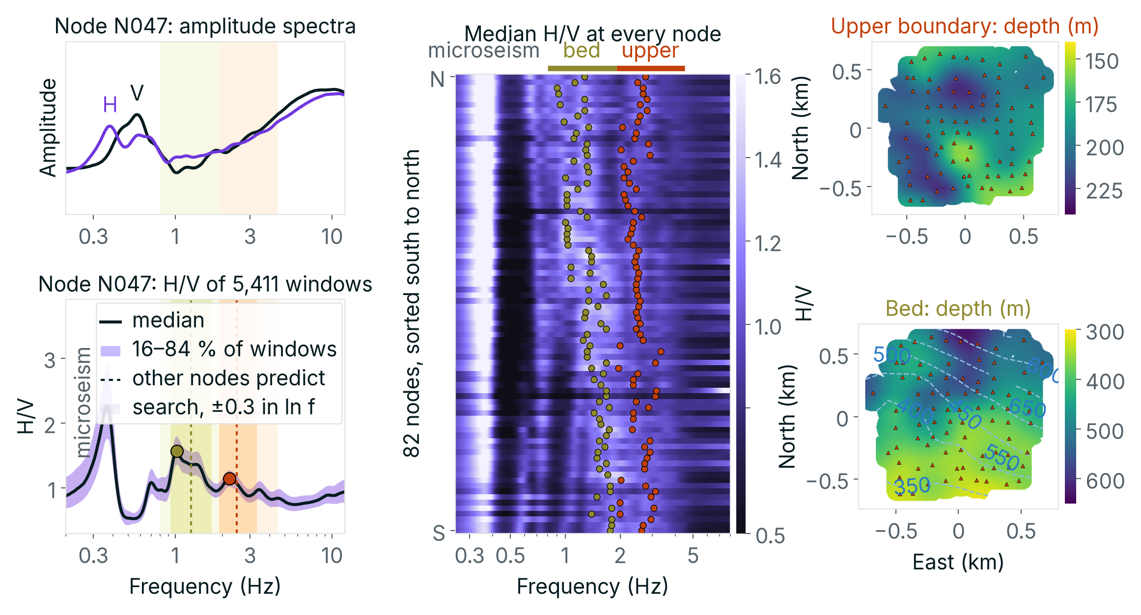
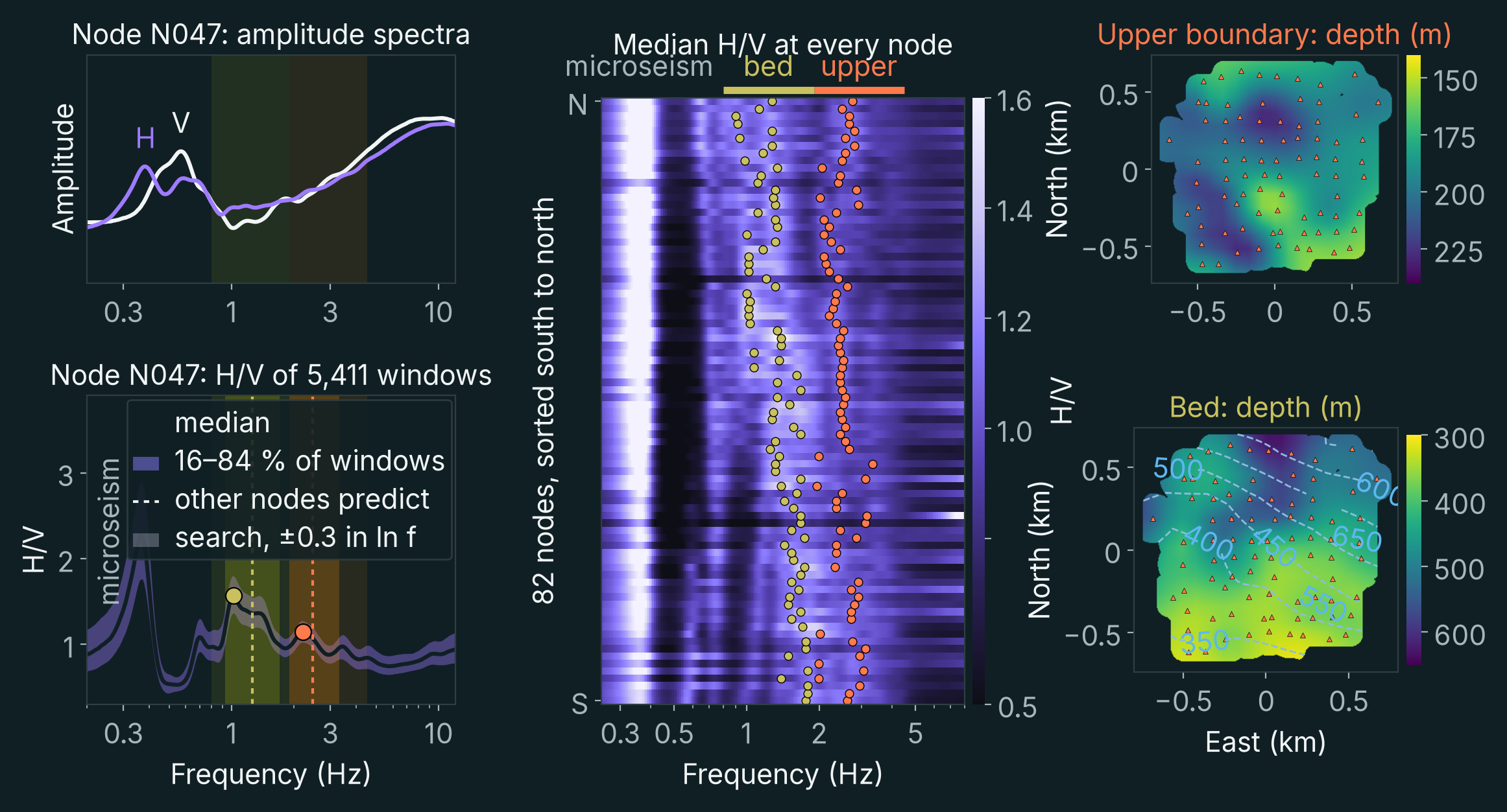
The close agreement between these independent observations showed that the seismic data could recover not only the average thickness of the ice but also important variations in the geometry of the underlying bedrock.
Step 3: dispersion and H/V peaks to refined interfaces
Ambient noise correlations provided surface-wave dispersion measurements across the array. HVSR measurements helped constrain the geometry of the interfaces within the ice and at its base.
Fitted together, the 54,469 Rayleigh- and Love-wave travel times between station pairs and the H/V peaks move both interfaces in 3-D, with the layer velocities held at their 1-D values. The bed deepens northward from 387 to 580 metres, a median 28 metres below the radar bed, which is not fitted (Figure 9).
Step 4: dispersion and local earthquakes to a 3-D velocity model
Recovering the bedrock interface was an important result, but the objective of seismic tomography is to reconstruct variations in seismic properties throughout a volume.
To achieve this, we also used local earthquakes recorded during the experiment.
Nearly 19,000 small seismic events were detected, most of them occurring within the upper 200 metres of ice. After locating and evaluating the events, 71 were retained for the inversion.
These earthquakes provided an additional source of information because their seismic waves travelled along paths different from those of the ambient surface waves. Some of these paths extended into the bedrock beneath the glacier (Figure 10).
Combining surface-wave measurements with the arrival times of compressional and shear waves from these events allowed us to construct a three-dimensional seismic velocity model.
Step 5: full-waveform inversion
We then applied full-waveform inversion (FWI), a technique that uses more of the information contained in the recorded seismic signals.
Conventional travel-time tomography attempts to reproduce the measured arrival times of seismic waves. Full-waveform inversion goes further by simulating the waveforms themselves and progressively modifying the velocity model to improve the agreement between simulated and observed signals.
In ambient noise FWI, each station serves as a virtual source. The correlations between its recording and those of every other station approximate the waveforms that an impulsive source at that station would produce (Figure 11). We used the vertical-component correlations of 79 virtual sources: 2,602 waveforms.
Each iteration of the inversion has three stages. First, a numerical simulation propagates the wavefield of every virtual source through the current model and computes the waveform expected at each station. Second, each simulated waveform is compared with the observed one; the misfit is the time shift that best aligns the two (Luo and Schuster 1991). Third, a second simulation, the adjoint, propagates these time shifts backwards from the stations. Combined with the first, it gives the sensitivity of the total misfit to the velocity at every point of the model (Tromp, Tape and Liu 2005), and the model is updated in the direction that reduces the misfit.
The method needs a good starting model. If a simulated waveform lags the observed one by more than half a period, the comparison can align the wrong cycles and push the model the wrong way, a problem known as cycle skipping. We therefore started from the model of step 4, and from the lowest frequencies, which have the longest periods: eight iterations at 2–7 Hz, then eight at 4–9 Hz, each band starting from the model of the one before.
Each iteration requires a forward and an adjoint simulation for every virtual source. The two frequency bands took about 20 and 22 GPU-hours on cloud GPUs.
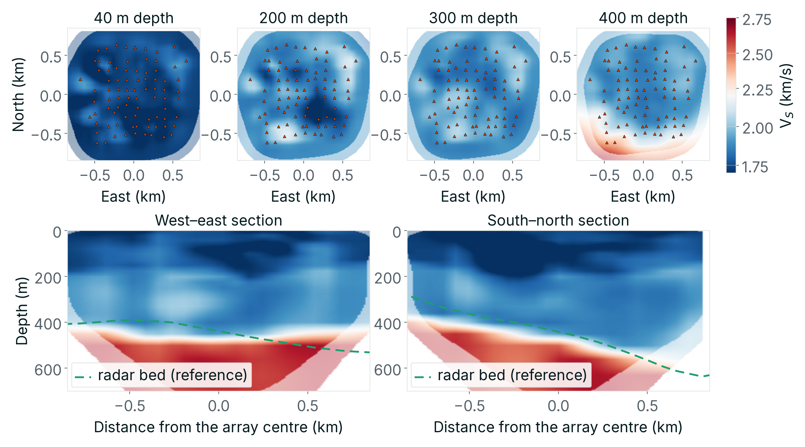
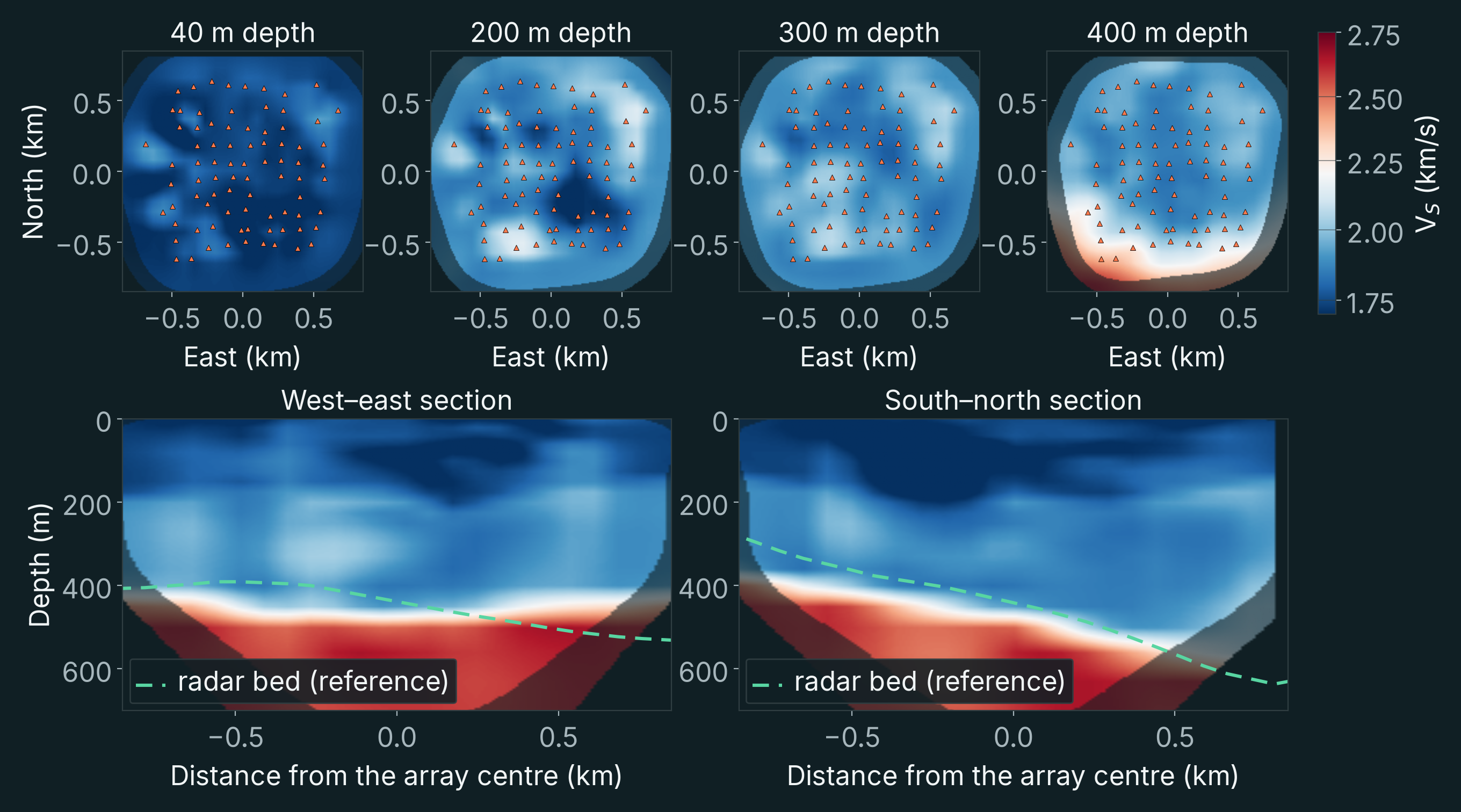
Using numerical simulations performed with SPECFEM3D, we refined the model through successive frequency bands. The waveform misfit decreased by 12% in the 2–7 Hz band and 28% in the 4–9 Hz band. Relative to the starting model, shear velocity changed by 2.3% (root mean square) where the data constrain it, and by 3–4% between 60 and 220 metres depth (Figure 12).
Drag the 3-D view to turn it, or step through the model with the slider.
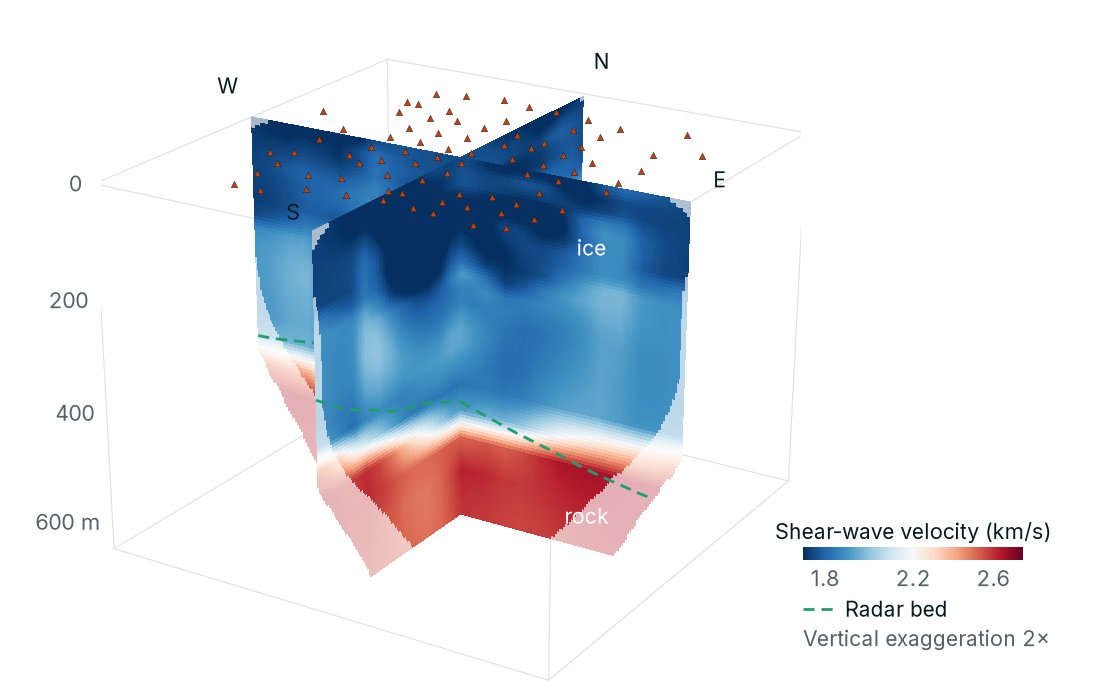
The final model recovered the ice–bedrock interface and provided information about seismic velocity immediately beneath it.
The results were consistent with the independent radar observations. In the three-dimensional interface inversion of step 3, the recovered bedrock surface lay a median of 28 metres below the radar-derived interface.
The experiment therefore demonstrated that passive seismic recordings could be used to reconstruct a three-dimensional velocity model beneath several hundred metres of ice. This answers the second question: the ice does not mask the ground below it.
What the seismic waves reveal about the ice
The measurements also revealed something interesting about the glacier itself.
Seismic velocity was not identical in every horizontal direction. Instead, it varied systematically with the direction of wave propagation.
This phenomenon, known as seismic anisotropy, occurs when the mechanical properties of a material depend on direction. It can result from aligned fractures, mineral fabrics or other directional structures.
Across the Greenland array, Rayleigh-wave velocities varied by approximately 2.5% with propagation direction, with larger variations in some parts of the glacier.
More importantly, the direction of slowest wave propagation was closely aligned with the direction perpendicular to surface crevasses. The average angular difference was approximately 10 degrees (Figure 13).
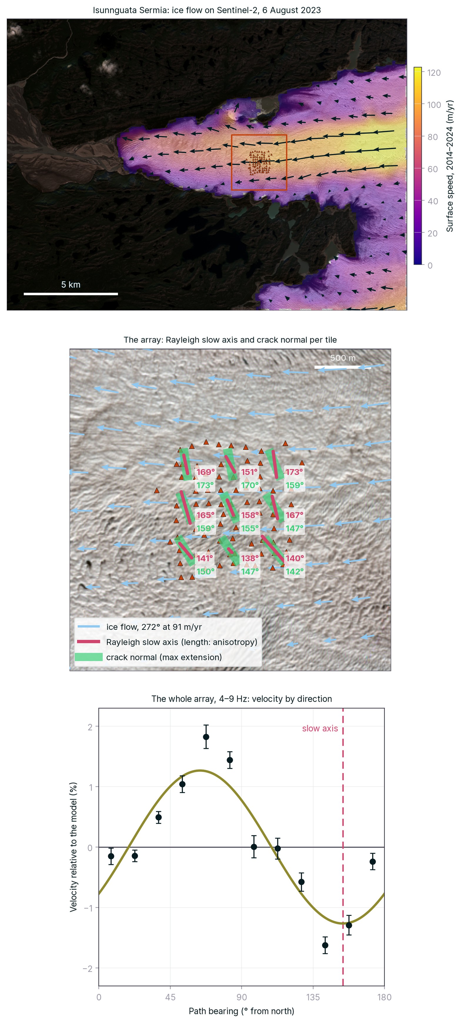
This relationship suggests that the seismic anisotropy reflects the fracture patterns and deformation of the ice.
Although our principal objective was to investigate the bedrock, the results show that the same passive seismic measurements can also provide information about the mechanical state of the overlying material.
The importance of survey design
The Greenland experiment demonstrated that seismic imaging beneath thick ice is possible, but it also illustrated an important limitation.
The array had originally been designed to study glacier dynamics, not deep geological structures. Its maximum aperture was approximately 1.6 kilometres.
The depth investigated by surface-wave tomography depends strongly on the wavelengths that can be measured. Longer wavelengths generally provide sensitivity to greater depths, but recovering them requires appropriate station spacing, array dimensions and usable low-frequency seismic energy.
In Greenland, the longest reliable Rayleigh wavelengths were approximately 1.3 kilometres (Figure 14).
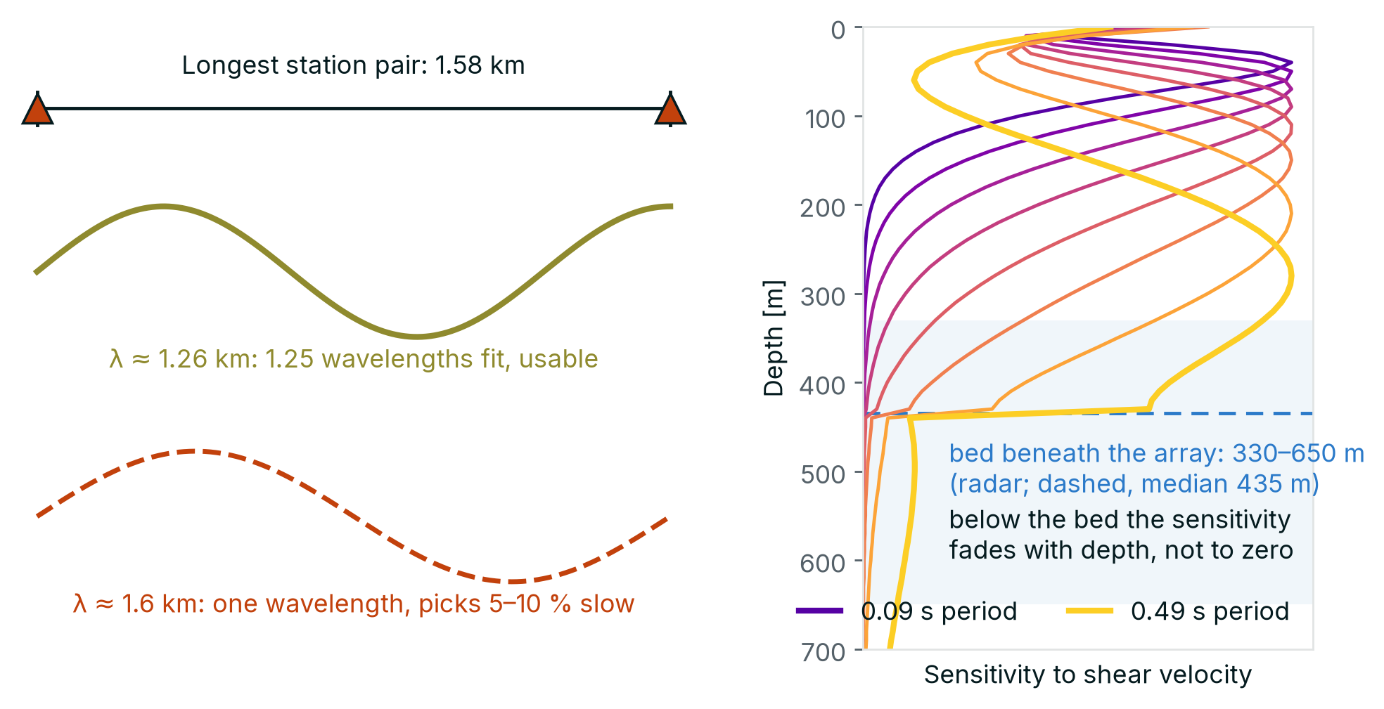
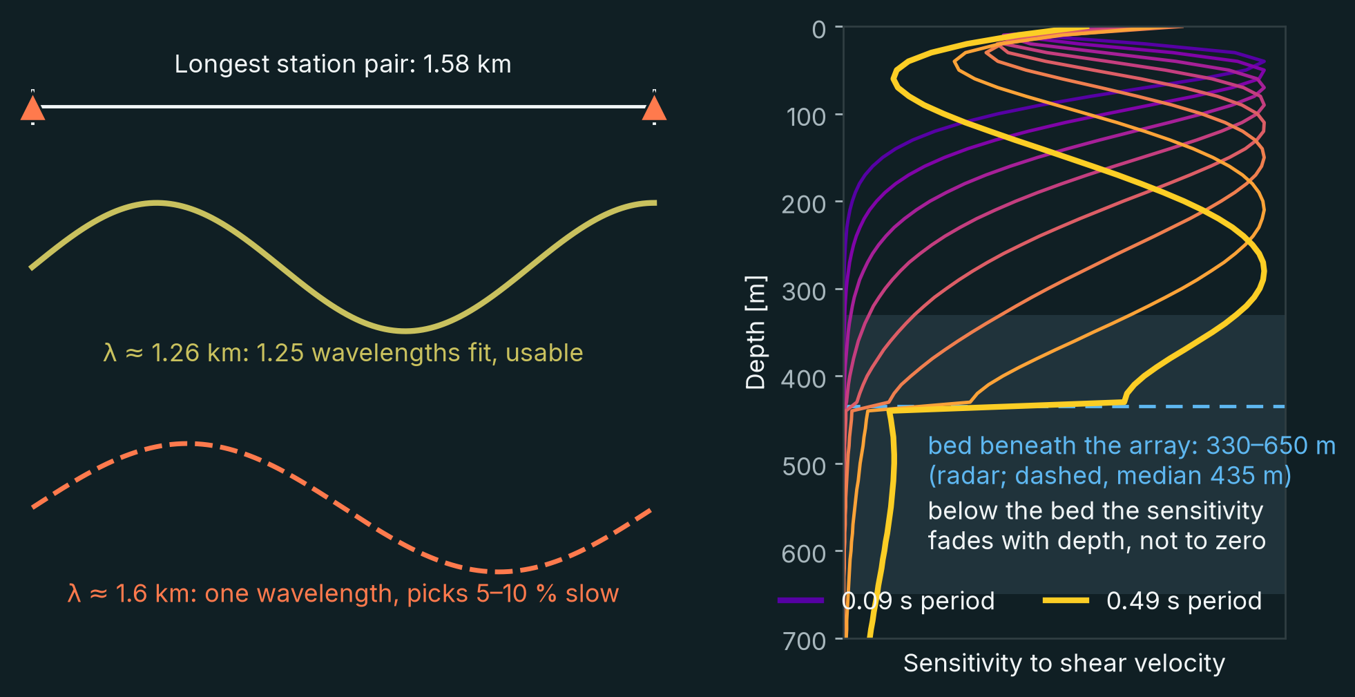
Consequently, the data provided useful information about the ice–bedrock interface and the rock immediately beneath it, but insufficient sensitivity to resolve geological variations deeper within the bedrock.
This is an important distinction. The experiment established that the ice itself did not prevent imaging of the underlying geology. It did not demonstrate that the particular array could resolve mineral deposits several kilometres beneath the glacier.
Investigating deeper structures would require an array designed for that purpose, with a larger aperture and measurements at longer periods.
The same principle applies to mineral exploration more generally. Survey design must reflect the depth, dimensions and physical properties of the geological structures being investigated.
Towards more effective exploration beneath cover
The study asked two questions of a glacier, and both answers are positive. The noise field recorded on the ice is good: strong across the band of interest, relatively homogeneous and arriving from many directions. And the ice is no impediment to the seismic waves: they pass through 330–650 metres of it and carry the signature of the rock below, so that the ice–rock transition recovered from the seismic data alone agrees with independent radar.
These results demonstrate that ambient noise tomography can image beneath the ice of a glacier. They do not demonstrate deep imaging of the rock: the array was designed to study the glacier, and its 1.6-kilometre aperture limits how far below the bed it can see. Nor is seismic velocity a direct measure of mineralization; its interpretation requires geological and other geophysical observations.
Ice is one example of cover. The method's requirements are the same beneath sediment, volcanic rock or glacial deposits: a good ambient noise field, and waves that reach the rock beneath the cover. Where they are met, ambient noise tomography needs no artificial source, records unattended in remote terrain, and maps seismic velocity in three dimensions to the depth that the array is designed for. That makes it a particularly efficient method of imaging the geology beneath cover, and of guiding where to drill.
About the research
This work was presented at the SEG Critical Minerals Forum in Vancouver, 27–29 October 2026, by Jean-Philippe Mercier, with Jubran Akram, Stephen Mosher and Noah Munro-Kagan (Concordens), and Nicolas Paris and Florent Gimbert (Université Grenoble Alpes).
The seismic data were acquired in 2023 by Université Grenoble Alpes and are publicly available through RESIF (network 9F, doi:10.15778/RESIF.9F2023). « F.G. and N.P. acknowledge funding from the European Research Council (ERC) under grant number 101126009 (REASSESS) ».
Selected references
- Schodde, R. (2025). Mineral deposit exploration—discovery trends: 1900–2023. SEG Discovery, 142, 19–35. doi:10.5382/Geo-and-Mining-28
- Paris, N., et al. (2026). Seismica, 5(2). doi:10.26443/seismica.v5i2.2557.
- Lindbäck, K., et al. (2014). High-resolution ice thickness and bed topography of a land-terminating section of the Greenland Ice Sheet. Earth System Science Data, 6, 331–338. doi:10.5194/essd-6-331-2014
- MacGregor, J. A., et al. (2024). Geophysical Research Letters. doi:10.1029/2023GL107357.
- Podolskiy, E. A., and Walter, F. (2016). Cryoseismology. Reviews of Geophysics, 54, 708–758. doi:10.1002/2016RG000526
- Dales, P., Audet, P., Olivier, G., and Mercier, J.-P. (2017). Interferometric methods for spatio-temporal seismic monitoring in underground mines. Geophysical Journal International, 210, 731–742. doi:10.1093/gji/ggx189
- Luo, Y., and Schuster, G. T. (1991). Wave-equation traveltime inversion. Geophysics, 56, 645–653. doi:10.1190/1.1443081
- Tromp, J., Tape, C., and Liu, Q. (2005). Seismic tomography, adjoint methods, time reversal and banana-doughnut kernels. Geophysical Journal International, 160, 195–216. doi:10.1111/j.1365-246X.2004.02453.x
What could your data reveal?
Discuss your geological objectives, existing recordings or next survey with our team.
Talk to Concordens